Beauty In Polar Coordinates

This post is a part of a series of guest-posts on polar coordinates and complex numbers. These posts were written by my pre-calc students:

Beauty in Polar Coordinates

by Luke VanDyke

Beauty can be found in mathematics in various places. Whether it be in Euler’s Identity or another beautiful equation of the sort, or in a magnificent graph, order and beauty are found on every page. One of the most interesting and amazing ways to graph objects is in polar form. A variety of shapes such as spirals, cardioids, and limaçon are just a few examples of the wide range of beauty found in graphing in the polar form. I think one of the most amazing curves that you can graph is the rose. Using Geogebra, I was able to explore in great deal the immense complexity of such an amazing curve and also notice several key patterns regarding the equation.



In order to fully demonstrate the beauty of the rose, I first inserted two sliders, a and b. I made the range for each slider from 0-10 with increments of .1. These sliders would serve as my values for a and n. The equation we learned in class (r=a*cos(nθ) and r=a*sin(θ)) must be changed into the curve expression on Geogebra. Mr. Roer helped me out a lot in converting to curve form. Once I had the equation in, I was able to play with the sliders and see how they worked. Slider A adjusts the size of the radius. The larger the number on the slider, the larger the rose will “grow”.

Slider B was a lot of fun to play with. Slider B adjusted the number and also the width of the “petals”. After playing around with both sliders, I noticed a pattern developing that affected the graph significantly. When the value of slider B was odd(let’s call this value x), the flower would have x number of petals. For example, if Slider B=1, there was just one circle. The same occurred for all other odd values between 0-10. On the other hand, even numbers also had an interesting pattern. For every even value between 0-10(we’ll call this value y), there would be 2y number of petals. For example, if 2 was the value on the B slider, the rose would have 4 petals.


This project was a really great opportunity to see God’s beauty as seen in mathematics. The saying “Out of intense complexities, intense simplicities emerge.” really goes hand in hand with this project. Once you put in the big, complex equation, a simplistic, beautiful image of a rose emerges. This saying also applies to roses in real life. Out of a complex equation of photosynthesis and many other factors, a beautiful flower emerges. There are many other examples all throughout God’s magnificent creation. Whether it be in the majestic landscapes throughout nature or in the complexity of infinitesimal human DNA and genetics, God’s awesome handiwork is seen all throughout the earth. Through this project, I’ve been able to reflect on how great God is and how everything in His creation is simply remarkable, even in places where you least expect it.

Transition Matrices

This post is a part of a series of guest-posts on the applications of matrix multiplication. These posts were written by my pre-calc students:

Transition Matrices

by Leanna Krueger 

Imagine that you own an apple orchard and you sell 3 different types of apples; Honeycrisp (A), Golden Delicious (B), and Gala (C). Honeycrisp apples sell the most while Golden Delicious is the runner up and Gala sells the least. You planted apple trees for each of these apples, and the cost of replacing each tree with the tree that produces apple A is too expensive until you get more money. In order to predict your earnings and decide when you can replant your orchard trees you need to estimate what people will buy. You know that this week the current market for apples is shown in the "state matrix" S shown below:

	A	B	C
Percentage of People Buying	60%	30%	10%

Suppose you surveyed repeated buyers and found the following:

A.                If people are buying A this week, the probability of them buying A next week is 70%. The probability of them buying B next week is 20% and the probability for C is 10%.

B.                 If people are buying B this week, the probability of them buying A next week is 50%. The probability of them buying B next week is 30% and the probability for C is 20%.

C.                 If people are buying C this week, the probability of them buying A next week is 30%. The probability of them buying B next week is 40% and the probability for purchasing C again is 30%.

You could set this information up in a transition matrix, T, shown below:

	A	B	C
A	.7	.2	.1
B	.5	.3	.2
C	.3	.4	.3

If a family was buying apple B, and you wanted to know the probability of them buying apple A 4 weeks later you would have to multiply the 2 matrices above forming S*T. After multiplying them once, you would have to multiply them a second time, and third time, and a fourth time. In a sense, doing that is the same thing as finding S*T to the fourth power:

	A	B	C
1 week	.6	.25	.15
2 weeks	.59	.255	.155
3 weeks	.587	.2565	.1565
4 weeks	.5861	.25695	.156951

Therefore, the probability of the family buying apple A 4 weeks later is 58.61%.  

Adjacency Matrices

This post is a part of a series of guest-posts on the applications of matrix multiplication. These posts were written by my pre-calc students:

Adjacency Matrices 

By John Taylor 

Let’s say you have to go over to your friend Will’s house, but you have to get some things done first. How can you know how many routes you can take and gets to Will’s? Enter the adjacency matrix. This helpful matrix can tell you how many different routes you can take of the same number of moves to get to the same place. Now the first thing you should do when you are starting to get ready to make your matrix is to look at your map:

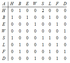
 Now figure out what these places are. The house is, well, your house. All the others, except W, are stores you need to go to: The sock shop (S), the book store (B), the library (L), the electronics store (E), the farmer’s market (F) and the drug store (D). The W is Will’s house. The next step is to write a matrix recording these relations. For each road from one place to another record a 1. If there is no connection put a zero. For a one-way street only write a 1 for the direction the arrow faces. If there are two options, say between home and the sock shop, enter a 2. This matrix will look like this.

Now we have this maps matrix. That was the hard part; now it’s quite simple. However many places you want to go to and raise the matrix to that power. (Note: This will give you all ways even if they repeat points. For the sake of this example you are very forgetful and often have to go back because you forgot many things at these stores.)

 Let’s go back to the trip to Will’s. You want to go to six places before you head over. Just raise the whole matrix to 6 and in the cell H,W you will see how many routes there are that reach Will’s in six moves. The resulting matrix will look like this:

Now look in the cell H,W and you will find out your answer. Even though most of the numbers are big, there are only 10 ways to get from your house to Will’s in 6 moves. This is the way adjacency matrices work. I hope this example has helped you understand these helpful matrices more fully.

Solving a systems of Equations with a Matrix

This post is a part of a series of guest-posts on the applications of matrix multiplication. These posts were written by my pre-calc students:

Systems of Equations Matrix Project

by Jake Melton

Matrices have many different applications and can be helpful in many situations. One such situation is solving systems of equations. Solving systems of equations using matrices takes several steps, all of which will be explained in the following blog post. All of the steps will be shown as if you were using a TI-89 calculator (or Mr. Roer's edits show steps for a TI-82, -83, -84). 

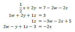
The following system of equations will be used as the example throughout the following post:

To begin the process we need to first write all of the equations in standard form (i.e. variables=number.) This will have to be done by hand. After we finish this process we get: 

Once we have written this new system of equations there are two ways we could go. First, we could complete the system of equations by hand. This process would include writing two matrices A and B. A would be a coefficient matrix, that is a matrix written using the number by which the variable is multiplied; this matrix would be 4 by 4. The second matrix, B would be a 4 by 1 matrix written using the answers. Remember, if there is no variable as seen in the second equation where there is no x, you must write a 0. The system of equations is then summarized by the matrix multiplication:

To find the solutions, you can simply multiply the inverse of A by B and the resulting 4 by 1 matrix would be the answers, illustrated here. 

*Note if the determinant of A equals zero the system has either no solution or many solutions. 

However, to solve the system of equations we could follow another much more simple process using our calculators. Using a TI-89 (or TI-82, -83, or-84) first press “on” and scroll up to the data/matrix editor  and press enter (or press 2nd Matrix). Select “new” then “matrix”. Next, enter the name you would like under “variable” and continue by pressing enter. The data should be empty, now simply enter your data into the table, making sure you enter a 4 by 5 matrix. This matrix is augmented [A|B] and will appear as follows. 

As you can see, this matrix is simply both matrices shown on the previous page combined. Now, simply press “enter” then “home”. Next you will need to click the “catalog” button found in the middle of your calculator, then press “2” and scroll to “rref(” and hit enter. (or press 2nd Matrix, over to calc, and down to B: rref ) Now you will need to enter the name of your matrix using “alpha” and the name of your matrix. The rref you just entered stands for “reduced row echelon form of a” or as Mr. Roer calls it, “really ridiculously easy form” and it simplifies the equations for you to give you:

Each row is a simplified equation. The first row simply means that 

1w +0x +0y +0z = 3.5  or, w = 3.5 

So now that you have found this matrix you can conclude that: 

w = 3.5 

x = -4 

y = -1.5 

z = 2.5 

These numbers shown above mean that w, x, y, and z are the only numbers that could be put into the original system of equations and make ALL of them true. And that is how you would go about finding the answer to a system of equations using matrices. Now you know how to solve these systems by hand or using your TI-89 calculator (or TI-82, -83, -84). Now use these steps to solve any difficult system of equations with ease. I hope you leave feeling enlightened and much smarter, or more confused, but hopefully the former.

Matrix Multiplication Cryptography

This post is a part of a series of guest-posts on the applications of matrix multiplication. These posts were written by my pre-calc students:

Matrix Cryptography
by David Stanley

Cryptography, put simply, is the art of encoding messages.  It serves to answer the simple question of how you get a message to a friend without your enemy being able to read it.  Cryptography has been used for centuries by militaries and intelligence agencies to send important messages, while insuring that the information the messages contain does not fall into enemy hands. 

Although there are many forms of cryptography, one of the simplest yet most effective forms of encryption still utilizes the simple matrix.The message is placed in matrix form, and then multiplied by a random square matrix or encoding matrix. 

 The first step is to write down the message that you wish to send.  I will use this completely true and totally non-brown nosing message as an example:

Mr Roer is the best math teacher ever in the history of humanity.

Secondly, you must create an encoding matrix.  This matrix must be a square matrix. An example of this would be:

In this kind of encryption, letters are assigned numbers for their place in the alphabet.  A would be 1, B would be 2, C would be 3 and so on.  Spaces are assigned the number 27, as their are only 26 letters in the alphabet.  So the message in matrix form would be:

Notice how my encoding matrix has the same amount of columns as the message matrix does rows.  This is required or else they cannot be multiplied.  All that is left to do is to multiply the encryption matrix by the message matrix.  This gives you:

Now if you received this in the mail, you would have no idea at all what it said.  In order to figure this out in a timely manner, you would have to have the decoding matrix.  The decoding matrix is the inverse of the encoding matrix.  This can easily be found on your calculator.  The decoding matrix for this problem is quite long, so I will round to four decimal places. 

The exact elements in the decoding matrix have more digits and would give the exact numbers as the original message. Using this rounded decryption matrix gives numbers that can all be rounded to the original message, though occasionally a letter might be slightly off.  

In summary, the encoding process written in calculator language when 

           [A] is the encoding matrix,

           [B] is the original message,  

    and [C] is the encoded message is [A]x[B]=[C]. 

The process of decoding the message is ([A]^-1)x[C]=[B]. 

And there you have it.  That is matrix cryptography in a nutshell. 

Meaningful Matrix Multiplication

This post is a part of a series of guest-posts on the applications of matrix multiplication. These posts were written by my pre-calc students:

The Christmas Party Competition by Kiera Suywn

Svetlana and Isabelle are frien-emies. Not only that, but they both love Christmas. Every year they each plan a Christmas party. This year their parties happened to be on the same day. So they are trying to beat each other out on who can get the best price for her party supplies. Svetlana needs 1 ½ gallon of eggnog, 6 twelve packs of candy canes, 3 gingerbread house kits, and 7 hot chocolate mixes. Isabelle needs 5 ½ gallons of eggnog, 2 twelve packs of candy canes, 7 gingerbread house making kits, and 4 hot chocolate mixes. They are both comparing prices from Meijer, Target, and Forest Hills Foods. To figure out who would have the best price at what store, they used matrices, something they learned a very long time ago in Pre-Calculus class and thought they would never use again.
Here is a chart showing the prices of the items per store. They put this as matrix [A] which is (stores x prices of food).

	Eggnog	Candy Canes	Gingerbread	Hot Chocolate
Target	2.79	2.49	9.99	1.99
Meijer	2.19	2.00	9.99	1.39
Forest Hills	3.99	1.25	7.99	4.99

            The next matrix they made was one that showed the (food x people) this went in the matrix [B] spot. 

	Svetlana	Isabelle
Eggnog	1	5
Candy Canes	6	2
Gingerbread house kit	3	7
Hot Chocolate	7	4

They multiplied these two matrices together which produced a (stores x people) matrix. This is what they got for their answers. This gave them the total amounts that each of their supplies would be.

	Svetlana	Isabelle
Target	89.49	112.74
Meijer	73.35	101.56
Forest Hills Foods	70.39	98.34

Forest Hills Foods had the best prices for both of them but Svetlana won by $27.95. Maybe next year Isabelle!